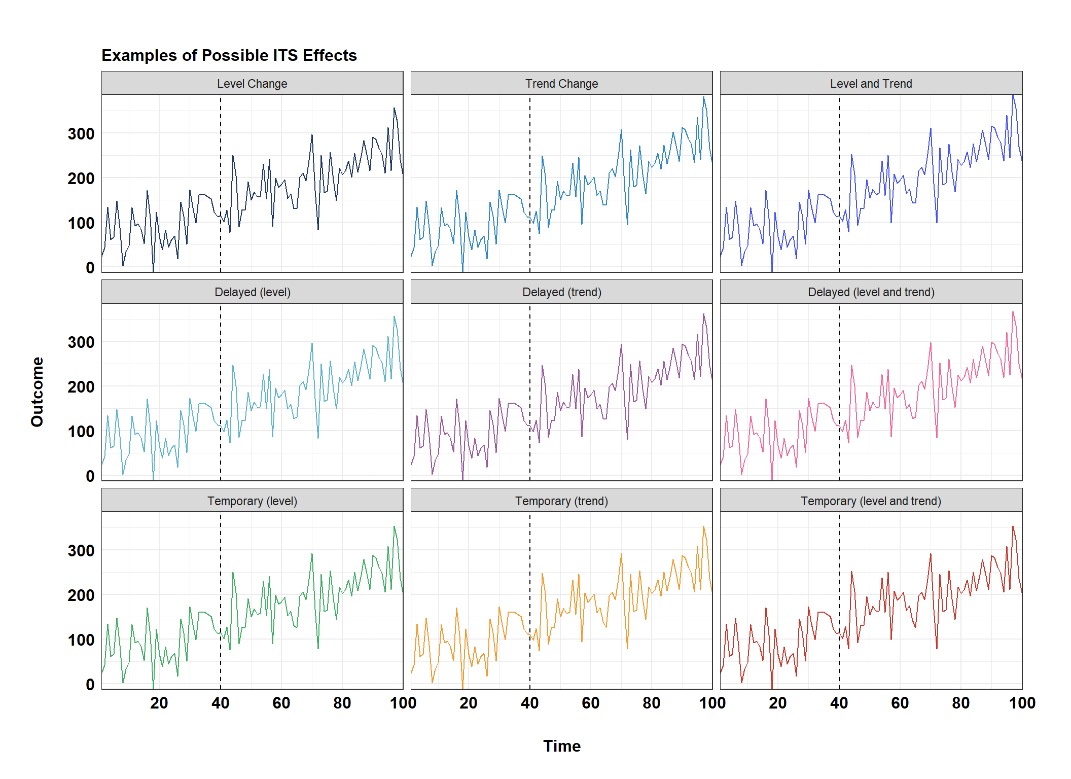
ITS analysis helps you pinpoint different ways a time series might be affected by an intervention.
Immediate Effect:
Represents a sudden shift in the data the moment the intervention takes place. Imagine a new policy leading to an abrupt change in behavior.
Did the intervention create an immediate spike or drop in the data?
Step Effect:
Reflects a permanent change in the baseline level of the time series. Think of stepping onto a higher or lower platform after the intervention – the overall level has shifted.
Did the intervention fundamentally alter the overall level of the time series?
Ramp Effect:
Demonstrates a gradual increase or decrease following the intervention. Picture yourself walking up or down a slope after the event – the trend and trajectory of the time series are constantly changing.
Did the intervention set in motion a gradual upward or downward trend?
ITS analysis isn’t just about single, isolated effects. The beauty of the method lies in its ability to capture a variety of ways the intervention might change the time series data:
Shifts & Slopes:
You can identify combinations of both immediate level changes (“step” effects) and changes in the trend of the data (“ramp” effects):
Level Only: Did the intervention create a jump or drop that then persists at a new, stable level?
Trend Only: Did the slope of the series gradually change direction over time after the intervention?
Both: An immediate change in the level, combined with a new upward or downward trend.
Delays:
In some cases, the full change caused by the intervention might not appear immediately. ITS can detect if an effect, whether a level shift or trend change, starts after a delay.
Temporary Changes:
Interventions don’t always have everlasting effects. Sometimes there’s a momentary shock and then a return to previous levels, or a brief trend change that flattens out again.
Below is a graphical visualization of potential different effects you might consider when designing an ITS analysis.
Understanding these combined effects gives you a richer picture of the intervention’s impact:
Magnitude: What was the combined influence on the overall level of your outcome?
Timing: Was the bulk of the impact immediate, delayed, or gradual?
Duration: Was the effect permanent or fleeting?
Source Code
# Defining Intervention EffectsITS analysis helps you pinpoint different ways a time series might be affected by an intervention.**Immediate Effect:**- Represents a sudden shift in the data the moment the intervention takes place. Imagine a new policy leading to an abrupt change in behavior.- Did the intervention create an immediate spike or drop in the data?**Step Effect:**- Reflects a permanent change in the baseline level of the time series. Think of stepping onto a higher or lower platform after the intervention – the overall level has shifted.- Did the intervention fundamentally alter the overall level of the time series?**Ramp Effect:**- Demonstrates a gradual increase or decrease following the intervention. Picture yourself walking up or down a slope after the event – the trend and trajectory of the time series are constantly changing.- Did the intervention set in motion a gradual upward or downward trend?ITS analysis isn't just about single, isolated effects. The beauty of the method lies in its ability to capture a variety of ways the intervention might change the time series data:- **Shifts & Slopes:** - You can identify combinations of both immediate level changes ("step" effects) and changes in the trend of the data ("ramp" effects): - **Level Only:** Did the intervention create a jump or drop that then persists at a new, stable level? - **Trend Only:** Did the slope of the series gradually change direction over time after the intervention? - **Both:** An immediate change in the level, combined with a new upward or downward trend.- **Delays:** - In some cases, the full change caused by the intervention might not appear immediately. ITS can detect if an effect, whether a level shift or trend change, starts after a delay.- **Temporary Changes:** - Interventions don't always have everlasting effects. Sometimes there's a momentary shock and then a return to previous levels, or a brief trend change that flattens out again.Below is a graphical visualization of potential different effects you might consider when designing an ITS analysis.```{r ITS-1,message = FALSE, warning=FALSE,error=FALSE,fig.dim = c(11, 8)}library(ggplot2)library(tidyverse)library(lubridate)# --- Parameters ----outcome_baseline <- 50 pre_intervention_slope <- 2 interv_point <- 40 n_timepoints <- 100 # --- Simulation ----set.seed(123) base_data <- tibble( time = 1:n_timepoints, outcome = outcome_baseline + pre_intervention_slope * time + rnorm(n_timepoints, 0, 50))# --- Functions to add effects ---level_change <- function(data, magnitude) { data$outcome[data$time >= interv_point] <- data$outcome[data$time >= interv_point] + magnitude return(data)}trend_change <- function(data, slope_change) { data$outcome[data$time >= interv_point] <- data$outcome[data$time >= interv_point] + slope_change * (data$time[data$time >= interv_point] - interv_point) return(data)}delayed_effect <- function(data, magnitude, delay, type = "level") { if(type == "level") { data$outcome[data$time >= (interv_point + delay)] <- data$outcome[data$time >= (interv_point + delay)] + magnitude } else { data$outcome[data$time >= (interv_point + delay)] <- data$outcome[data$time >= (interv_point + delay)] + slope_change * (data$time[data$time >= (interv_point + delay)] - (interv_point + delay)) } return(data)}temporary_effect <- function(data, magnitude, duration, type = "level") { if (type == "level") { data$outcome[data$time >= interv_point & data$time < (interv_point + duration)] <- data$outcome[data$time >= interv_point & data$time < (interv_point + duration)] + magnitude } else { start_trend <- interv_point end_trend <- interv_point + duration data$outcome[data$time >= start_trend & data$time < end_trend] <- data$outcome[data$time >= start_trend & data$time < end_trend] + magnitude * (data$time[data$time >= start_trend & data$time < end_trend] - start_trend) } return(data)}# --- Scenarios ------# 1. Level change onlydf_level <- level_change(base_data, magnitude = 4)# 2. Slope change onlydf_trend <- trend_change(base_data , slope_change = 0.5)# 3. Level and Slope changedf_both <- level_change(df_trend, magnitude = 4)# 4. Delaysslope_change = 0.3df_delayed_level <- delayed_effect(base_data, magnitude = 4, delay = 25)df_delayed_trend <- delayed_effect(base_data, magnitude = 0.5, delay = 25, "trend")df_delayed_both <- delayed_effect(df_delayed_trend, magnitude = 4, delay = 25)# 5. Temporary changesdf_temp_level <- temporary_effect(base_data , magnitude = 4, duration = 25)df_temp_trend <- temporary_effect(base_data , magnitude = 0.5, duration = 25, type="trend")df_temp_both <- temporary_effect(df_temp_trend , magnitude = 4, duration = 25)df_effects <- dplyr::bind_rows( dplyr::mutate(df_level,effects = "Level Change", order = 1), dplyr::mutate(df_trend,effects = "Trend Change", order = 2), dplyr::mutate(df_both,effects = "Level and Trend", order = 3), dplyr::mutate(df_delayed_level,effects = "Delayed (level)", order = 4), dplyr::mutate(df_delayed_trend,effects = "Delayed (trend)", order = 5), dplyr::mutate(df_delayed_both,effects = "Delayed (level and trend)", order = 6), dplyr::mutate(df_temp_level,effects = "Temporary (level)", order = 7), dplyr::mutate(df_temp_trend,effects = "Temporary (trend)", order = 8), dplyr::mutate(df_temp_both,effects = "Temporary (level and trend)", order = 9) )# --- Plotting -----ggplot(df_effects, aes(x = time, y = outcome, color = fct_reorder(effects, order), group = fct_reorder(effects, order), fill = fct_reorder(effects, order))) + geom_line() + geom_vline(xintercept = interv_point, linetype = "dashed") + facet_wrap(vars(fct_reorder(effects, order)), nrow = 3) + theme_bw() + theme( # White background areas panel.background = element_rect(fill = "white"), plot.background = element_rect(fill = "white"), plot.margin = unit(c(0.5, 0.5, 0.5, 0.5), "inches"), # Plot margins plot.title = element_text( size = 12, face = "bold", color = "black" ), axis.title.y = element_text( size = 12, face = "bold", color = "black", vjust = 7 ), axis.title.x = element_text( size = 12, face = "bold", color = "black", vjust = -7 ), axis.text.y = element_text( face = "bold", size = 12, color = "black" ), axis.text.x = element_text( face = "bold", color = "black", size = 12, angle = 0, vjust = 1 ), # Remove axis ticks axis.ticks = element_blank(), legend.position = "none" ) + ggtitle("Examples of Possible ITS Effects") + ylab("Outcome") + scale_y_continuous(expand = c(0, 0),breaks = scales::pretty_breaks()) + scale_x_continuous(expand = c(0, 0),breaks = scales::pretty_breaks()) + xlab("Time") + scale_color_manual(values= c("#203864", "#3086c3", "#4754eb", "#5fb4cc" ,"#985b9a", "#ee6c9b", "#42ae65", "#ef9c33", "#c23a2e", "#b06d18"),aesthetics = "colour") + scale_color_manual(values= c("#203864", "#3086c3", "#4754eb", "#5fb4cc" ,"#985b9a", "#ee6c9b", "#42ae65", "#ef9c33", "#c23a2e", "#b06d18"),aesthetics = "fill") ```Understanding these combined effects gives you a richer picture of the intervention's impact:- **Magnitude:** What was the combined influence on the overall level of your outcome?- **Timing:** Was the bulk of the impact immediate, delayed, or gradual?- **Duration:** Was the effect permanent or fleeting?